NBA Playoff Predictions

Neel Shah

Table of contents

  1. Introduction
    1.1. Background Information
    1.2. Objective
    1.3. Configuration
  2. Data Collection
    2.1. Data Sources
    2.2. Scraping Data
  3. Data Processing
    3.1. Cleaning Data
    3.1.1. Renaming a Single Column
    3.1.2. Renaming All Columns
    3.1.3. Cleaning a CSV File
    3.2. Merging Data
    3.3. Filtering Rows
    3.4. Setting Data Types
    3.5. Adding New Columns
    3.5.1. Determining Conferences
    3.5.2. Determining Playoff Seeding
    3.5.3. Converting Team Records to Winning Percentages
    3.6. Labeling Columns
    3.7. Looking at Tidy Data
  4. Exploratory Data Analysis & Visualization
    4.1. Setup
    4.1.1. Splitting Data
    4.1.2. Making Subplots
    4.2. Correlating Individual Statistics With Playoff Wins
    4.2.1. Overall Rating
    4.2.2. Offensive Volume
    4.2.3. Offensive Efficiency
    4.2.4. Rebounding
    4.2.5. Passing/Turnovers
    4.2.6. Defensive
    4.2.7. Remarks
    4.3. The Efficiency Landscape
    4.4. Combining Common Predictors: Seed and True Shooting Percentage
  5. Modeling: Analysis, Hypothesis Testing, & Machine Learning
    5.1. Problem Definition
    5.2. Splitting Data
    5.3. Machine Learning Pipelines
    5.3.1. Preprocessing Data
    5.3.2. Feature Selection / Dimensionality Reduction
    5.3.3. Model Selection / Hyperparameter Tuning
    5.4. Evaluating Models
    5.4.1. Comparing Models
    5.4.2. Diving Deeper
    5.4.3. Predicting the $2023$ NBA Playoffs
  6. Interpretation: Insight & Policy Decision

1. Introduction

Let's start off by providing some background information about this topic, defining the objectives of this project, and configuring some things.

1.1. Background Information

The National Basketball Association (NBA) is a professional basketball league in the United States. There are $30$ teams in the league, divided evenly into $2$ conferences: the Eastern Conference and the Western Conference.

In the regular season, each team plays $82$ games. NBA regular season standings are determined by teams' win-loss records within their conferences.

The top $8$ teams from each conference advance to the playoffs. In the event of a tie in the standings, there is a tie-breaking procedure used to determine playoff seeding.

Starting in the $2019\text{-}20$ season, the NBA added a play-in tournament to give the $9^\text{th}$ and $10^\text{th}$ place teams in each conference the opportunity to earn a spot in the playoffs. It works as follows:

  • The $7^\text{th}$ and $8^\text{th}$ place teams play a game to determine the $7^\text{th}$ seed. The winner advances to the playoffs.
  • The $9^\text{th}$ and $10^\text{th}$ place teams play an elimination game. The loser is eliminated.
  • The loser of the $7/8$ game and the winner of the $9/10$ game play an elimination game to determine the $8^\text{th}$ seed. The winner advances to the playoffs; the loser is eliminated.

Once the final playoff seeding is determined, each team plays an opponent in a best-of-$7$ series. The first to win $4$ games advances to the next round. The first round is followed by the conference semifinals, then the conference finals, then the finals. The team that wins the NBA Finals is the NBA Champion.

The matchups for each round are determined using a traditional bracket structure, shown below:
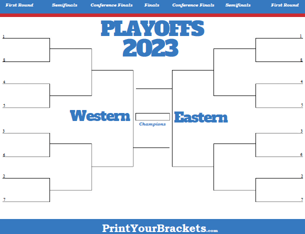
NBA Playoff Bracket

1.2. Objective

We want to perform some analysis to see if we can identify factors underlying teams' level of success in the playoffs. Our ultimate goal will be to predict the outcome of the NBA Playoffs using data from the regular season.

Can we accurately predict how many playoff games a team will win?

With this information, we could determine if a team is likely to:

  • Make the conference semifinals (i.e. win at least $4$ playoff games)
  • Make the conference finals (i.e. win at least $8$ playoff games)
  • Make the finals (i.e. win at least $12$ playoff games)
  • Win the championship (i.e. win $16$ playoff games)

These are some of the questions we want to answer as we go through the full data science pipeline.

1.3. Configuration

We'll start by importing the Python libraries necessary for this project and configuring some things.

In [ ]:
# system
import warnings
import time
from pathlib import Path
import itertools
import textwrap

# data
import requests
from bs4 import BeautifulSoup, Comment, MarkupResemblesLocatorWarning
import pandas as pd
import numpy as np

# visualization
import plotly.io as pio
import plotly.express as px
import plotly.graph_objects as go
from plotly.subplots import make_subplots

# modeling
from sklearn.model_selection import train_test_split, GridSearchCV
from sklearn.pipeline import Pipeline
from sklearn.compose import ColumnTransformer
from sklearn.preprocessing import (
    OneHotEncoder,
    StandardScaler,
    MinMaxScaler,
    MaxAbsScaler,
    RobustScaler,
)
from sklearn.feature_selection import RFECV
from sklearn.linear_model import LinearRegression, Ridge, Lasso, ElasticNet
from sklearn.tree import DecisionTreeRegressor, plot_tree
from sklearn.ensemble import (
    RandomForestRegressor,
    GradientBoostingRegressor,
    AdaBoostRegressor,
)
from sklearn.metrics import r2_score, mean_squared_error, mean_absolute_error
import skops.io as sio

# warnings
warnings.filterwarnings("ignore", category=MarkupResemblesLocatorWarning, module="bs4")

# requests
headers = {
    "User-Agent": "Mozilla/5.0 (Windows NT 10.0; Win64; x64) AppleWebKit/537.36 (KHTML, like Gecko) Chrome/110.0.0.0 Safari/537.36"
}

# pandas
pd.set_option("display.max_columns", None)

# plotly
pio.renderers.default = "notebook+plotly_mimetype+png+jpeg+svg+pdf"

2. Data Collection

Now, we need to collect data that we can use in our analysis.

2.1. Data Sources

We will will scrape data from Basketball Reference, a site that provides historical basketball data.

We will use data from the $2002\text{-}03$ season (when the NBA switched to the current playoff format, where every series is best-of-$7$) to the $2022\text{-}23$ season (the current season). For each season, we will scrape the following information:

  • Per Game Stats from Season Summary page
  • Advanced Stats from Season Summary page
  • Expanded Standings from Standings page
  • Advanced Stats from Playoffs Summary page

For convenience, we will define a function called pages_to_scrape. Given a season, it will return a dictionary which maps the URL of the page we will be scraping to the list of information about each table we will be scraping from that page.

Each element in the list will be in the form of a dictionary with $2$ items:

  • The id of the HTML table element we will be scraping from the page
  • The path where we will be storing the table as a CSV
In [ ]:
def pages_to_scrape(season):
    return {
        f"https://www.basketball-reference.com/leagues/NBA_{season}.html": [
            {
                "id": "per_game-team",
                "path": f"data/raw/{season}/regular_season/per_game_stats.csv",
            },
            {
                "id": "advanced-team",
                "path": f"data/raw/{season}/regular_season/advanced_stats.csv",
            },
        ],
        f"https://www.basketball-reference.com/leagues/NBA_{season}_standings.html": [
            {
                "id": "expanded_standings",
                "path": f"data/raw/{season}/regular_season/standings.csv",
            }
        ],
        f"https://www.basketball-reference.com/playoffs/NBA_{season}.html": [
            {
                "id": "advanced-team",
                "path": f"data/raw/{season}/playoffs/advanced_stats.csv",
            }
        ],
    }

2.2. Scraping Data

To scrape the data from each page, we will do the following:

  • Perform an HTTP GET request to the appropriate URL using the Requests library.
  • Parse the webpage using Beautiful Soup.
  • Find the HTML table with the appropriate id.
  • Read the parsed HTML table into a DataFrame using pandas.
  • Ensure that the appropriate path exists in the filesystem using pathlib.
  • Write the DataFrame to a CSV file at the appropriate path using pandas.

In our approach, there are a few issues that we have to address as well:

  • To save time, if the CSV files for a page already exist, we will not re-scrape the page.
  • It appears that some of the table elements are hidden inside of HTML comments, so we have to look there if a table can't be found normally.
  • To avoid hitting rate limits (from making too many requests in a given time period), we have to add a $10$ second sleep between each HTTP GET request using the time library.
In [ ]:
# get list of seasons
seasons = list(range(2003, 2023 + 1))

# go through seasons
for season in seasons:

    # get pages to scrape for season
    pages = pages_to_scrape(season)

    # go through pages
    for url, infoList in pages.items():

        # skip if all CSV files exist
        if all([Path(info["path"]).exists() for info in infoList]):
            continue

        # request data from page
        page = requests.get(url, headers=headers)
        soup = BeautifulSoup(page.content, "html.parser")

        # go through tables
        for info in infoList:

            # skip if CSV file exists
            if Path(info["path"]).exists():
                continue

            # find table
            table = soup.find("table", id=info["id"])
            if table is None:
                for comment in soup.find_all(
                    string=lambda text: isinstance(text, Comment)
                ):
                    comment_soup = BeautifulSoup(comment, "html.parser")
                    table = comment_soup.find("table", id=info["id"])
                    if table is not None:
                        break

            # convert table to DataFrame and save as CSV
            df = pd.read_html(str(table))[0]
            Path(info["path"]).parent.mkdir(parents=True, exist_ok=True)
            df.to_csv(info["path"], index=False)

        # sleep for 10 seconds before next request
        time.sleep(10)

3. Data Processing

Now that we have collected all the data, we need to process it and make it suitable for analysis. We will be making extensive use of pandas for manipulating DataFrames.

3.1. Cleaning Data

The first step is to figure out how we will be cleaning all the data.

3.1.1. Renaming a Single Column

First, let's define a function called rename_column. It will take in a column name and return a column name that has been modified to provide more consistency.

The renaming rules are as follows:

  • If the column name contains Unnamed, then we will replace it with a blank string.
  • If the column name is Rk, then we will replace it with Rank.
  • If the column name is Tm, then we will replace it with Team.
  • If the column name is Offense Four Factors (which is the name for a group of $4$ different columns), then we will replace it with a blank string. This way, the sub-columns will be assumed to be referring to the team's statistics on offense.
  • If the column name is Defense Four Factors (which is the name for a group of $4$ different columns), then we will replace it with Opp. This way, the sub-columns will be assumed to be referring to the opponent's statistics on offense (the team's statistics on defense).
  • Otherwise, we will return the original name.
In [ ]:
def rename_column(name):
    if "Unnamed" in name:
        return ""
    elif name == "Rk":
        return "Rank"
    elif name == "Tm":
        return "Team"
    elif name == "Offense Four Factors":
        return ""
    elif name == "Defense Four Factors":
        return "Opp"
    else:
        return name

3.1.2. Renaming All Columns

Now, let's define a function called rename_columns. It takes in a DataFrame and a list of the header rows.

It works as follows:

  • If there is a single header row, then it renames each column by calling rename_column.
  • If there are multiple header rows, then it renames both names for each column by calling rename_column and combines them.
In [ ]:
def rename_columns(df, header):
    if len(header) == 1:
        df.columns = [rename_column(i) for i in df.columns]
    else:
        df.columns = [f"{rename_column(i)}{rename_column(j)}" for i, j in df.columns]
    return df

3.1.3. Cleaning a CSV File

Now, let's create a dictionary called files_to_clean with information about the CSV files we need to clean. It will map the file name to a dictionary with $2$ items:

  • The header of the CSV file (an array of the row indices for the header)
  • The columns of the CSV file that we want to keep (after they have been renamed using the rename_columns function above)
  • The column_mappings, which map old column names to new column names (for renaming purposes)
In [ ]:
files_to_clean = {
    "regular_season/per_game_stats.csv": {
        "header": [0],
        "columns": [
            "Team",
            "FG",
            "FGA",
            "FG%",
            "3P",
            "3PA",
            "3P%",
            "2P",
            "2PA",
            "2P%",
            "FT",
            "FTA",
            "FT%",
            "ORB",
            "DRB",
            "TRB",
            "AST",
            "STL",
            "BLK",
            "TOV",
            "PF",
            "PTS",
        ],
        "column_mappings": {},
    },
    "regular_season/advanced_stats.csv": {
        "header": [0, 1],
        "columns": [
            "Team",
            "SRS",
            "ORtg",
            "DRtg",
            "NRtg",
            "Pace",
            "FTr",
            "3PAr",
            "TS%",
            "eFG%",
            "TOV%",
            "ORB%",
            "FT/FGA",
            "OppeFG%",
            "OppTOV%",
            "OppDRB%",
            "OppFT/FGA",
        ],
        "column_mappings": {"OppDRB%": "DRB%"},
    },
    "regular_season/standings.csv": {
        "header": [0, 1],
        "columns": [
            "Rank",
            "Team",
            "Overall",
            "PlaceHome",
            "PlaceRoad",
            "ConferenceE",
            "ConferenceW",
        ],
        "column_mappings": {
            "Overall": "OverallRecord",
            "PlaceHome": "HomeRecord",
            "PlaceRoad": "RoadRecord",
            "ConferenceE": "EastRecord",
            "ConferenceW": "WestRecord",
        },
    },
    "playoffs/advanced_stats.csv": {
        "header": [0, 1],
        "columns": ["Rank", "Team", "W", "L"],
        "column_mappings": {"Rank": "PlayoffRank", "W": "PlayoffW", "L": "PlayoffL"},
    },
}

Now, let's define a function called clean_csv. Given the path to a CSV file, it will return a DataFrame with a cleaned version of the data from the CSV file.

To clean a file, we do the following:

  • Using the files_to_clean dictionary, obtain the information needed to clean the CSV file at the specified path.
  • Read the CSV file at the specified path into a DataFrame.
  • Do an initial renaming of columns by calling the rename_columns function.
  • Keep only the specified columns of the DataFrame.
  • Rename the remaining columns using the specified column_mappings.
  • Remove any rows where the Team is League Average (since this is an aggregate of all the rows in the DataFrame, and we have no use for it).
  • Remove the * character for any values in the Team column (since it is used to indicate if a team made the playoffs, but we already have that data).
  • Replace Seattle Supersonics with Seattle SuperSonics and Charlotte Bobcats with Charlotte Hornets in the Team column (to account for inconsistent naming of teams in the CSV files).
In [ ]:
def clean_csv(path):

    # obtain information needed to clean CSV file
    name = f"{Path(path).parents[0].name}/{Path(path).name}"
    info = files_to_clean[name]

    # read CSV file
    df = pd.read_csv(path, header=info["header"])

    # rename columns
    rename_columns(df, info["header"])

    # remove unnecessary columns
    df = df[info["columns"]]

    # rename remaining columns
    df = df.rename(columns=info["column_mappings"])

    # remove "League Average" row
    df = df[df["Team"] != "League Average"]

    # remove "*" from team names
    df["Team"] = df["Team"].str.replace("*", "", regex=False)

    # make team names consistent
    df["Team"] = df["Team"].str.replace(
        "Seattle Supersonics", "Seattle SuperSonics", regex=False
    )
    df["Team"] = df["Team"].str.replace(
        "Charlotte Bobcats", "Charlotte Hornets", regex=False
    )

    # return DataFrame
    return df

3.2. Merging Data

Now, we need to merge all the cleaned data into a single DataFrame.

For each season, we will do the following:

  • Clean the $4$ CSV files for the season using the clean_csv function.
  • Merge the $4$ DataFrames for the season on the Team column using an outer join.
  • Add a Season column to the beginning of the DataFrame and fill all of the rows with the same season value.

Then, we concatenate the DataFrames for each season into a single DataFrame.

In [ ]:
# create main DataFrame
data = pd.DataFrame()

# go through seasons
for season in seasons:

    # initialize season DataFrame
    season_data = None

    # get list of CSV files for season
    infoList = list(itertools.chain(*pages_to_scrape(season).values()))
    pathList = [info["path"] for info in infoList]

    # go through CSV files
    for index, path in enumerate(pathList):

        # clean CSV file and store as DataFrame
        df = clean_csv(path)

        # merge DataFrame with season DataFrame
        if index == 0:
            season_data = df
        else:
            season_data = season_data.merge(df, on="Team", how="outer")

    # add season column at beginning
    season_data.insert(0, "Season", season)

    # add season DataFrame to main DataFrame
    data = pd.concat(objs=[data, season_data])

Now, we can look at the merged data.

In [ ]:
data.info()
<class 'pandas.core.frame.DataFrame'>
Int64Index: 628 entries, 0 to 29
Data columns (total 48 columns):
 #   Column         Non-Null Count  Dtype  
---  ------         --------------  -----  
 0   Season         628 non-null    int64  
 1   Team           628 non-null    object 
 2   FG             628 non-null    float64
 3   FGA            628 non-null    float64
 4   FG%            628 non-null    float64
 5   3P             628 non-null    float64
 6   3PA            628 non-null    float64
 7   3P%            628 non-null    float64
 8   2P             628 non-null    float64
 9   2PA            628 non-null    float64
 10  2P%            628 non-null    float64
 11  FT             628 non-null    float64
 12  FTA            628 non-null    float64
 13  FT%            628 non-null    float64
 14  ORB            628 non-null    float64
 15  DRB            628 non-null    float64
 16  TRB            628 non-null    float64
 17  AST            628 non-null    float64
 18  STL            628 non-null    float64
 19  BLK            628 non-null    float64
 20  TOV            628 non-null    float64
 21  PF             628 non-null    float64
 22  PTS            628 non-null    float64
 23  SRS            628 non-null    float64
 24  ORtg           628 non-null    float64
 25  DRtg           628 non-null    float64
 26  NRtg           628 non-null    float64
 27  Pace           628 non-null    float64
 28  FTr            628 non-null    float64
 29  3PAr           628 non-null    float64
 30  TS%            628 non-null    float64
 31  eFG%           628 non-null    float64
 32  TOV%           628 non-null    float64
 33  ORB%           628 non-null    float64
 34  FT/FGA         628 non-null    float64
 35  OppeFG%        628 non-null    float64
 36  OppTOV%        628 non-null    float64
 37  DRB%           628 non-null    float64
 38  OppFT/FGA      628 non-null    float64
 39  Rank           628 non-null    int64  
 40  OverallRecord  628 non-null    object 
 41  HomeRecord     628 non-null    object 
 42  RoadRecord     628 non-null    object 
 43  EastRecord     628 non-null    object 
 44  WestRecord     628 non-null    object 
 45  PlayoffRank    340 non-null    float64
 46  PlayoffW       340 non-null    float64
 47  PlayoffL       340 non-null    float64
dtypes: float64(40), int64(2), object(6)
memory usage: 240.4+ KB
In [ ]:
data
Out[ ]:
Season Team FG FGA FG% 3P 3PA 3P% 2P 2PA 2P% FT FTA FT% ORB DRB TRB AST STL BLK TOV PF PTS SRS ORtg DRtg NRtg Pace FTr 3PAr TS% eFG% TOV% ORB% FT/FGA OppeFG% OppTOV% DRB% OppFT/FGA Rank OverallRecord HomeRecord RoadRecord EastRecord WestRecord PlayoffRank PlayoffW PlayoffL
0 2003 Dallas Mavericks 38.5 85.1 0.453 7.8 20.3 0.381 30.8 64.8 0.475 18.1 21.9 0.829 11.1 31.0 42.1 22.4 8.1 5.5 11.6 21.1 103.0 7.90 110.7 102.3 8.4 92.5 0.257 0.239 0.543 0.498 10.9 25.4 0.213 0.473 14.8 70.9 0.221 1 60-22 33-8 27-14 26-4 34-18 8.0 10.0 10.0
1 2003 Golden State Warriors 37.3 84.6 0.441 5.2 15.1 0.344 32.1 69.6 0.462 22.6 29.0 0.778 15.7 31.0 46.7 20.9 7.2 6.2 15.8 21.8 102.4 -0.60 108.3 109.5 -1.2 94.2 0.343 0.178 0.526 0.472 13.9 35.0 0.267 0.482 12.2 67.9 0.220 19 38-44 24-17 14-27 19-11 19-33 NaN NaN NaN
2 2003 Sacramento Kings 39.5 85.2 0.464 6.0 15.7 0.381 33.5 69.5 0.482 16.7 22.3 0.746 11.0 33.5 44.5 24.8 9.0 5.6 14.5 20.3 101.7 6.68 105.9 99.1 6.8 95.4 0.262 0.184 0.535 0.499 13.3 25.6 0.196 0.446 13.6 70.6 0.204 3 59-23 35-6 24-17 23-7 36-16 3.0 7.0 5.0
3 2003 Los Angeles Lakers 37.7 83.6 0.451 5.9 16.7 0.356 31.8 66.9 0.475 19.0 26.0 0.734 13.1 31.1 44.3 23.3 7.8 5.7 14.5 22.9 100.4 2.71 107.2 104.7 2.5 92.5 0.311 0.199 0.528 0.486 13.3 30.2 0.228 0.477 13.4 72.7 0.241 6 50-32 31-10 19-22 17-13 33-19 7.0 6.0 6.0
4 2003 Milwaukee Bucks 37.1 81.3 0.457 7.1 18.6 0.383 30.0 62.7 0.478 18.1 23.3 0.776 10.7 28.9 39.5 22.2 7.6 4.2 12.7 22.2 99.5 -0.24 108.8 108.6 0.2 90.4 0.287 0.229 0.543 0.500 12.2 25.6 0.222 0.494 13.5 69.9 0.237 16 42-40 25-16 17-24 32-22 10-18 11.0 2.0 4.0
... ... ... ... ... ... ... ... ... ... ... ... ... ... ... ... ... ... ... ... ... ... ... ... ... ... ... ... ... ... ... ... ... ... ... ... ... ... ... ... ... ... ... ... ... ... ... ... ...
25 2023 Orlando Magic 40.5 86.3 0.470 10.8 31.1 0.346 29.8 55.2 0.539 19.6 25.0 0.784 10.2 33.1 43.2 23.2 7.4 4.7 15.1 20.1 111.4 -2.39 111.6 114.2 -2.6 99.3 0.290 0.361 0.573 0.532 13.4 23.8 0.227 0.550 13.1 77.7 0.211 25 34-48 20-21 14-27 20-32 14-16 NaN NaN NaN
26 2023 Charlotte Hornets 41.3 90.4 0.457 10.7 32.5 0.330 30.5 57.9 0.528 17.6 23.6 0.749 11.0 33.5 44.5 25.1 7.7 5.2 14.2 20.3 111.0 -5.89 109.2 115.3 -6.1 100.8 0.261 0.360 0.550 0.516 12.3 23.8 0.195 0.544 12.5 75.5 0.211 27 27-55 13-28 14-27 15-37 12-18 NaN NaN NaN
27 2023 Houston Rockets 40.6 88.9 0.457 10.4 31.9 0.327 30.2 56.9 0.530 19.1 25.3 0.754 13.4 32.9 46.3 22.4 7.3 4.6 16.2 20.5 110.7 -7.62 111.4 119.3 -7.9 99.0 0.285 0.359 0.554 0.516 14.0 30.2 0.215 0.564 11.8 75.8 0.218 28 22-60 14-27 8-33 10-20 12-40 NaN NaN NaN
28 2023 Detroit Pistons 39.6 87.1 0.454 11.4 32.4 0.351 28.2 54.6 0.516 19.8 25.7 0.771 11.2 31.3 42.4 23.0 7.0 3.8 15.1 22.1 110.3 -7.73 110.7 118.9 -8.2 99.0 0.295 0.372 0.561 0.520 13.3 24.9 0.227 0.557 11.9 74.0 0.231 30 17-65 9-32 8-33 8-44 9-21 NaN NaN NaN
29 2023 Miami Heat 39.2 85.3 0.460 12.0 34.8 0.344 27.3 50.5 0.540 19.1 23.0 0.831 9.7 30.9 40.6 23.8 8.0 3.0 13.5 18.5 109.5 -0.13 113.0 113.3 -0.3 96.3 0.270 0.408 0.574 0.530 12.4 22.8 0.224 0.561 14.5 77.7 0.198 13 44-38 27-14 17-24 24-28 20-10 4.0 3.0 1.0

628 rows × 48 columns

3.3. Filtering Rows

We want to analyze teams' level of success in the playoffs, so it only makes sense to consider teams that made the playoffs in our analysis.

Thus, we will drop rows where the PlayoffRank, PlayoffW, or PlayoffL columns are NaN.

We will also drop rows where the sum of PlayoffW and PlayoffL is $0$ (which would indicate that a team made it to the play-in tournament, but did not advance to the playoffs).

In [ ]:
data = data.dropna(subset=["PlayoffRank", "PlayoffW", "PlayoffL"])
data = data[(data["PlayoffW"] != 0) | (data["PlayoffL"] != 0)]
data = data.reset_index(drop=True)

3.4. Setting Data Types

As we can see, most of the columns in the DataFrame have the correct dtypes, but there are a few we need to correct. Specifically, PlayoffRank, PlayoffW, and PlayoffL need to be changed from float64 to int64.

In [ ]:
data = data.astype({"PlayoffRank": "int64", "PlayoffW": "int64", "PlayoffL": "int64"})

3.5. Adding New Columns

Now, using our existing data, we want to add a few new columns to our DataFrame that will be useful in analysis.

3.5.1. Determining Conferences

One important column the data is missing is Conference. It will be useful to know which conference a team is in, because that determines playoff matchups.

The EastRecord and WestRecord columns are in the form W-L (where W is the number of wins and L is the number of losses), indicating a team's record against opponents in each conference. We can calculate the number of games a team played in each conference using the formula below:

$$ \text{games} = \text{wins} + \text{losses} $$

Then, we can determine a team's Conference by checking if the team played more games in the East or the West.

In [ ]:
def get_conference(row):
    east_wins, east_losses = row["EastRecord"].split("-")
    west_wins, west_losses = row["WestRecord"].split("-")
    east_games = int(east_wins) + int(east_losses)
    west_games = int(west_wins) + int(west_losses)
    return "East" if east_games > west_games else "West"


data.insert(2, "Conference", data.apply(get_conference, axis=1))

3.5.2. Determining Playoff Seeding

Another important column the data is missing is Seed. This is likely to be important, because playoff seeding determines the matchups. As you can imagine, the $1^\text{st}$ seed is typically expected to win more games than the $8^\text{th}$ seed, so this is an important column to include.

We can determine the playoff seeding by doing the following:

  • Group the data by Season and then Conference.
  • Rank each team by its overall Rank within the group.

This should give us a Seed between $1$ (referred to as the highest seed) and $8$ (referred to as the lowest seed).

In [ ]:
data.insert(
    3,
    "Seed",
    data.groupby(["Season", "Conference"])["Rank"]
    .rank(method="dense", ascending=True)
    .astype("int64"),
)

3.5.3. Converting Team Records to Winning Percentages

Currently, we have $5$ columns that have team record in the form of W-L (where W is the number of wins and L is the number of losses): OverallRecord, HomeRecord, RoadRecord, EastRecord, and WestRecord.

We want to standardize these columns by turning them into winning percentages using the formula below:

$$ \text{winning percentage} = \frac{\text{wins}}{\text{wins} + \text{losses}} $$

This will give us $5$ new columns to replace the existing ones: W%, HomeW%, RoadW%, EastW%, and WestW%.

In [ ]:
def record_to_win_pct(record):
    wins, losses = record.split("-")
    return int(wins) / (int(wins) + int(losses))


for (win_pct, record) in [
    ("W%", "OverallRecord"),
    ("HomeW%", "HomeRecord"),
    ("RoadW%", "RoadRecord"),
    ("EastW%", "EastRecord"),
    ("WestW%", "WestRecord"),
]:
    data[record] = data[record].apply(record_to_win_pct)
    data = data.rename(columns={record: win_pct})

Now that we know each team's Conference as well as its winning percentage against teams from each conference, let's add a column named ConferenceW%, which is a team's winning percentage against teams in its own conference.

In [ ]:
data.insert(
    len(data.columns) - 3,
    "ConferenceW%",
    data.apply(
        lambda row: row["EastW%"] if row["Conference"] == "East" else row["WestW%"],
        axis=1,
    ),
)

3.6. Labeling Columns

Since there are so many columns in our DataFrame, it can be difficult to see what each one means. For this reason, we will create a dictionary named data_labels mapping each column name to a label describing it. We can use these labels later on (e.g. in our plots).

In [ ]:
data_labels = {
    "Season": "Season",
    "Team": "Team",
    "Conference": "Conference",
    "Seed": "Seed",
    "FG": "Field Goals (FG)",
    "FGA": "Field Goal Attempts (FGA)",
    "FG%": "Field Goal Percentage (FG%)",
    "3P": "3-Point Field Goals (3P)",
    "3PA": "3-Point Field Goal Attempts (3PA)",
    "3P%": "3-Point Field Goal Percentage (3P%)",
    "2P": "2-Point Field Goals (2P)",
    "2PA": "2-Point Field Goal Attempts (2PA)",
    "2P%": "2-Point Field Goal Percentage (2P%)",
    "FT": "Free Throws (FT)",
    "FTA": "Free Throw Attempts (FTA)",
    "FT%": "Free Throw Percentage (FT%)",
    "ORB": "Offensive Rebounds (ORB)",
    "DRB": "Defensive Rebounds (DRB)",
    "TRB": "Total Rebounds (TRB)",
    "AST": "Assists (AST)",
    "STL": "Steals (STL)",
    "BLK": "Blocks (BLK)",
    "TOV": "Turnovers (TOV)",
    "PF": "Personal Fouls (PF)",
    "PTS": "Points (PTS)",
    "SRS": "Simple Rating System (SRS)",
    "ORtg": "Offensive Rating (ORtg)",
    "DRtg": "Defensive Rating (DRtg)",
    "NRtg": "Net Rating (NRtg)",
    "Pace": "Pace Factor (Pace)",
    "FTr": "Free Throw Attempt Rate (FTr)",
    "3PAr": "3-Point Attempt Rate (3PAr)",
    "TS%": "True Shooting Percentage (TS%)",
    "eFG%": "Effective Field Goal Percentage (eFG%)",
    "TOV%": "Turnover Percentage (TOV%)",
    "ORB%": "Offensive Rebound Percentage (ORB%)",
    "FT/FGA": "Free Throws Per Field Goal Attempt (FT/FGA)",
    "OppeFG%": "Opponent Effective Field Goal Percentage (OppeFG%)",
    "OppTOV%": "Opponent Turnover Percentage (OppTOV%)",
    "DRB%": "Defensive Rebound Percentage (DRB%)",
    "OppFT/FGA": "Opponent Free Throws Per Field Goal Attempt (OppFT/FGA)",
    "Rank": "Rank",
    "W%": "Winning Percentage",
    "HomeW%": "Home Winning Percentage",
    "RoadW%": "Road Winning Percentage",
    "EastW%": "East Winning Percentage",
    "WestW%": "West Winning Percentage",
    "ConferenceW%": "Conference Winning Percentage",
    "PlayoffRank": "Playoff Rank",
    "PlayoffW": "Playoff Wins",
    "PlayoffL": "Playoff Losses",
}

3.7. Looking at Tidy Data

Now, our data should be nice and tidy, making it suitable for analysis. Let's take a quick look before moving on.

In [ ]:
data
Out[ ]:
Season Team Conference Seed FG FGA FG% 3P 3PA 3P% 2P 2PA 2P% FT FTA FT% ORB DRB TRB AST STL BLK TOV PF PTS SRS ORtg DRtg NRtg Pace FTr 3PAr TS% eFG% TOV% ORB% FT/FGA OppeFG% OppTOV% DRB% OppFT/FGA Rank W% HomeW% RoadW% EastW% WestW% ConferenceW% PlayoffRank PlayoffW PlayoffL
0 2003 Dallas Mavericks West 1 38.5 85.1 0.453 7.8 20.3 0.381 30.8 64.8 0.475 18.1 21.9 0.829 11.1 31.0 42.1 22.4 8.1 5.5 11.6 21.1 103.0 7.90 110.7 102.3 8.4 92.5 0.257 0.239 0.543 0.498 10.9 25.4 0.213 0.473 14.8 70.9 0.221 1 0.731707 0.804878 0.658537 0.866667 0.653846 0.653846 8 10 10
1 2003 Sacramento Kings West 3 39.5 85.2 0.464 6.0 15.7 0.381 33.5 69.5 0.482 16.7 22.3 0.746 11.0 33.5 44.5 24.8 9.0 5.6 14.5 20.3 101.7 6.68 105.9 99.1 6.8 95.4 0.262 0.184 0.535 0.499 13.3 25.6 0.196 0.446 13.6 70.6 0.204 3 0.719512 0.853659 0.585366 0.766667 0.692308 0.692308 3 7 5
2 2003 Los Angeles Lakers West 5 37.7 83.6 0.451 5.9 16.7 0.356 31.8 66.9 0.475 19.0 26.0 0.734 13.1 31.1 44.3 23.3 7.8 5.7 14.5 22.9 100.4 2.71 107.2 104.7 2.5 92.5 0.311 0.199 0.528 0.486 13.3 30.2 0.228 0.477 13.4 72.7 0.241 6 0.609756 0.756098 0.463415 0.566667 0.634615 0.634615 7 6 6
3 2003 Milwaukee Bucks East 7 37.1 81.3 0.457 7.1 18.6 0.383 30.0 62.7 0.478 18.1 23.3 0.776 10.7 28.9 39.5 22.2 7.6 4.2 12.7 22.2 99.5 -0.24 108.8 108.6 0.2 90.4 0.287 0.229 0.543 0.500 12.2 25.6 0.222 0.494 13.5 69.9 0.237 16 0.512195 0.609756 0.414634 0.592593 0.357143 0.592593 11 2 4
4 2003 Orlando Magic East 8 35.9 82.5 0.436 6.9 19.4 0.357 29.0 63.1 0.460 19.7 25.4 0.777 11.7 29.2 40.9 20.4 8.5 3.7 14.4 23.0 98.5 -0.39 105.2 105.0 0.2 93.1 0.307 0.235 0.526 0.478 13.3 27.0 0.239 0.486 15.1 71.1 0.250 17 0.512195 0.634146 0.390244 0.574074 0.392857 0.574074 15 3 4
... ... ... ... ... ... ... ... ... ... ... ... ... ... ... ... ... ... ... ... ... ... ... ... ... ... ... ... ... ... ... ... ... ... ... ... ... ... ... ... ... ... ... ... ... ... ... ... ... ... ... ...
331 2023 Phoenix Suns West 4 42.1 90.1 0.467 12.2 32.6 0.374 29.9 57.5 0.520 17.2 21.7 0.793 11.8 32.4 44.2 27.3 7.1 5.3 13.5 21.2 113.6 2.08 115.1 113.0 2.1 98.2 0.241 0.362 0.570 0.535 12.0 26.6 0.191 0.532 12.9 76.0 0.234 10 0.548780 0.682927 0.414634 0.500000 0.576923 0.576923 3 4 1
332 2023 Los Angeles Clippers West 6 41.1 86.1 0.477 12.7 33.4 0.381 28.4 52.7 0.539 18.7 23.9 0.781 9.8 33.4 43.2 23.9 7.1 4.4 14.2 19.5 113.6 0.31 115.0 114.5 0.5 98.0 0.278 0.387 0.588 0.551 12.8 22.9 0.217 0.543 11.7 76.6 0.195 12 0.536585 0.560976 0.512195 0.566667 0.519231 0.519231 14 1 4
333 2023 Brooklyn Nets East 6 41.5 85.1 0.487 12.8 33.8 0.378 28.7 51.3 0.559 17.7 22.1 0.800 8.2 32.3 40.5 25.5 7.1 6.2 13.7 21.1 113.4 1.03 115.0 114.1 0.9 98.3 0.260 0.397 0.598 0.562 12.7 19.6 0.208 0.530 12.2 73.7 0.212 9 0.548780 0.560976 0.536585 0.576923 0.500000 0.576923 16 0 4
334 2023 Cleveland Cavaliers East 4 41.6 85.2 0.488 11.6 31.6 0.367 30.0 53.6 0.559 17.5 22.5 0.780 9.7 31.4 41.1 24.9 7.1 4.7 13.3 19.0 112.3 5.23 116.1 110.6 5.5 95.7 0.264 0.371 0.590 0.556 12.3 23.6 0.206 0.535 14.4 76.3 0.210 5 0.621951 0.756098 0.487805 0.653846 0.566667 0.653846 10 1 3
335 2023 Miami Heat East 7 39.2 85.3 0.460 12.0 34.8 0.344 27.3 50.5 0.540 19.1 23.0 0.831 9.7 30.9 40.6 23.8 8.0 3.0 13.5 18.5 109.5 -0.13 113.0 113.3 -0.3 96.3 0.270 0.408 0.574 0.530 12.4 22.8 0.224 0.561 14.5 77.7 0.198 13 0.536585 0.658537 0.414634 0.461538 0.666667 0.461538 4 3 1

336 rows × 51 columns

4. Exploratory Data Analysis & Visualization

Now, it is time to explore some of the trends in this data through data visualization. We will be making extensive use of Plotly for data visualization.

4.1. Setup

Before we start creating visualizations, there are a few things we need to set up.

4.1.1. Splitting Data

Since the $2023$ playoffs are still ongoing, let's split our data into $2$ DataFrames: past_data and current_data. We will only use past_data for now.

In [ ]:
past_data = data[data["Season"] < 2023]
current_data = data[data["Season"] == 2023]

4.1.2. Making Subplots

Since there are lots of columns in our DataFrame, we will be creating lots of graphs that make use of subplots.

For convenience, we will define a function named get_subplots.

It takes in:

  • df: a DataFrame with our data
  • labels: a dictionary mapping column names to descriptions to use as labels
  • X_names: a list of columns we want to use as the $x$-axis of a subplot
  • y_name: the name of the column we want to use as the $y$-axis for every subplot
  • rows: the number of rows in the overall figure
  • cols: the number of columns in the overall figure.

It will return a $\text{rows} \times \text{cols}$ figure with plots of y_name vs. x_name for every x_name in X_names using the data in df.

We will also add a regression line to each subplot using the linear regression (ordinary least squares) model from scikit-learn.

In [ ]:
def get_subplots(df, labels, X_names, y_name, rows, cols):

    # create subplot titles
    titles = []
    width = 30
    for x_name in X_names:
        title = f"{labels[y_name]} vs. {labels[x_name]}"
        title = "<br>".join(textwrap.wrap(title, width=width))
        titles.append(title)

    # create figure with subplots
    fig = make_subplots(rows=rows, cols=cols, subplot_titles=titles)

    # go through each subplot
    for (index, x_name) in enumerate(X_names):

        # get row and column of subplot
        row = index // cols + 1
        col = index % cols + 1

        # create hovertemplate for subplot
        hovertemplate = "<br>".join(
            [
                "%{xaxis.title.text}=%{x}",
                "%{yaxis.title.text}=%{y}",
                "Team=%{customdata[0]}",
                "Season=%{customdata[1]}",
            ]
        )

        # create subplot
        subplot = go.Scatter(
            x=df[x_name],
            y=df[y_name],
            mode="markers",
            customdata=df[["Team", "Season"]],
            hovertemplate=hovertemplate,
            name="",
            showlegend=False,
        )

        # add subplot to figure
        fig.add_trace(subplot, row, col)
        fig.update_xaxes(title_text=labels[x_name], row=row, col=col)
        fig.update_yaxes(title_text=labels[y_name], row=row, col=col)

        # compute regression line for subplot
        model = LinearRegression()
        X = df[[x_name]].values
        y = df[y_name]
        model.fit(X, y)
        equation = f"y = {model.intercept_:.2f} + {model.coef_[0]:.2f}x"
        score = model.score(X, y)
        x_range = np.linspace(df[x_name].min(), df[x_name].max(), 100)
        y_range = model.predict(x_range.reshape(-1, 1))

        # create regression line for subplot
        line = go.Scatter(
            x=x_range,
            y=y_range,
            mode="lines",
            hovertemplate=f"{equation}<br>r^2 = {score}",
            name="Regression Line",
            showlegend=False,
            line={"color": "black"},
        )

        # add regression line for subplot to figure
        fig.add_trace(line, row, col)

    # update figure layout
    fig.update_layout(height=rows * 400)

    # return figure
    return fig

4.2. Correlating Individual Statistics With Playoff Wins

As we can see, there are quite a lot of statistics in the DataFrame, so we will group them into the following categories:

  • Overall Rating
  • Offensive Volume
  • Offensive Efficiency
  • Rebounding
  • Passing/Turnovers
  • Defensive

Our goal is to see which statistics in each category are most correlated with playoff wins. Are there any statistics that individually work as decent predictors of playoff wins (even with just a simple linear regression model)? Or do we need to look at statistics together to make any sense of the data?

We will be making scatter plots of playoff wins vs. each statistic in each category, with regression lines added. This is just meant for preliminary analysis, as linear regression is probably overly simplistic when looking at most of these statistics. However, these plots might give us some helful intuition for understanding the data.

4.2.1. Overall Rating

We'll start with some statistics that provide an overall rating of a team:

  • Rank (Rank): ranking within league, by win-loss record
  • Seed (Seed): placement in the playoff bracket (ranking within conference, by win-loss record)
  • Simple Rating System (SRS): team rating that takes into account average point differential and strength of schedule
  • Net Rating (NRtg): point differential (difference between points produced and allowed) per $100$ possessions
  • Winning Percentage (W%): percentage of games won
  • Home Winning Percentage (HomeW%): percentage of games won in home games
  • Road Winning Percentage (RoadW%): percentage of games won in road games
  • East Winning Percentage (EastW%): percentage of games won vs. Eastern Conference teams
  • West Winning Percentage (WestW%): percentage of games won vs. Western Conference teams
  • Conference Winning Percentage (ConferenceW%): percentage of games won vs. teams within conference
In [ ]:
overall_rating_stats = [
    "Rank",
    "Seed",
    "SRS",
    "NRtg",
    "W%",
    "HomeW%",
    "RoadW%",
    "EastW%",
    "WestW%",
    "ConferenceW%",
]
fig = get_subplots(past_data, data_labels, overall_rating_stats, "PlayoffW", 4, 3)
fig.show()

As we can see from the scatter plots, all of these statistics show some correlation with winning percentage (even though the relation might not be linear).

In particular, the following statistics seem like the best predictors of playoff wins:

  • Rank (Rank)
  • Seed (Seed)
  • Net Rating (NRtg)
  • Winning Percentage (W%)
  • Conference Winning Percentage (ConferenceW%)

It's particularly interesting that conference winning percentage seems to be more tightly correlated with playoff wins than home/road/East/West winning percentage.

4.2.2. Offensive Volume

Now, we'll look at some offensive statistics that are volume-based (i.e. based on the number of shots made):

  • Field Goals (FG): number of $3$-point and $2$-point shots made
  • $3$-Point Field Goals (3P): number of $3$-point shots (taken outside the $3$-point line) made
  • $2$-Point Field Goals (2P): number of $2$-point shots (taken inside the $3$-point line) made
  • Free Throws (FT): number of free throws (penalty shots awarded after free throws) made
  • Points (PTS): number of points scored ($1$ point per free throw, $2$ points per $2$-point field goal, and $3$ points per $3$-point field goal)
In [ ]:
offensive_volume_stats = ["FG", "3P", "2P", "FT", "PTS"]
fig = get_subplots(past_data, data_labels, offensive_volume_stats, "PlayoffW", 2, 3)
fig.show()

Based on the scatter plots, there appears to be little to no correlation between any of these statistics and playoff wins. This is not very surprising, considering that scoring has high variability.

Perhaps, offensive volume statistics will only be useful when paired with offensive efficiency statistics.

4.2.3. Offensive Efficiency

Now, we'll look at some offensive statistics that are efficiency-based (i.e. based on points per possession or shot attempt):

  • Field Goal Percentage (FG%): ratio of field goals made to field goals attempted
  • 3-Point Field Goal Percentage (3P%): ratio of $3$-point field goals made to $3$-point field goals attempted
  • 2-Point Field Goal Percentage (2P%): ratio of $2$-point field goals made to $2$-point field goals attempted
  • Free Throw Percentage (FT%): ratio of free throws made to free throws attempted
  • True Shooting Percentage (TS%): measure of shooting efficiency that accounts for all $3$ methods of scoring (free throws, $2$-point field goals, and $3$-point field goals)
  • Effective Field Goal Percentage (eFG%): measure of shooting efficiency that accounts for $3$-point field goals being worth more than $2$-point field goals
  • Free Throw Rate (FTr): number of free throw attempts per field goal attempt (measures team's ability to draw fouls and get to free throw line)
  • $3$-Point Attempt Rate (3PAr): number of $3$-point field goal attempts per field goal attempt (measures team's ability to score from deep, which has become more important during the $3$-point revolution)
  • Free Throws Per Field Goal Attempt (FT/FGA): number of free throws made per field goal attempt (measures team's ability to get to free throw line and make free throws)
  • Pace (Pace): offensive possessions per game
  • Offensive Rating (ORtg): points produced per $100$ possessions
In [ ]:
offensive_efficiency_stats = [
    "FG%",
    "3P%",
    "2P%",
    "FT%",
    "TS%",
    "eFG%",
    "FTr",
    "3PAr",
    "FT/FGA",
    "Pace",
    "ORtg",
]
fig = get_subplots(past_data, data_labels, offensive_efficiency_stats, "PlayoffW", 4, 3)
fig.show()

As we can see from the scatter plots, a few of these statistics show some correlation with playoff wins (even though the relation might not be linear).

In particular, the following statistics seem like the best predictors of playoff wins:

  • True Shooting Percentage (TS%)
  • Effective Field Goal Percentage (eFG%)
  • Offensive Rating (ORtg)

However, none of these statistics seem like good predictors of playoff wins on their own (since the scatter plots show very weak correlation). Perhaps, offensive efficiency statistics will only be useful when paired with offensive volume statistics.

4.2.4. Rebounding

Now, we'll look at some rebounding statistics:

  • Total Rebounds (TRB): number of rebounds on offense and defense
  • Offensive Rebounds (ORB): number of rebounds on offense
  • Defensive Rebounds (DRB): number of rebounds on defense
  • Offensive Rebound Percentage (ORB%): percentage of offensive rebounds team got
  • Defensive Rebounds Percentage (DRB%): percentage of defensive rebounds team got
In [ ]:
rebounding_stats = ["TRB", "ORB", "DRB", "ORB%", "DRB%"]
fig = get_subplots(past_data, data_labels, rebounding_stats, "PlayoffW", 2, 3)
fig.show()

Based on the scatter plots, there appears to be little to no correlation between any of these statistics and playoff wins. This is not very surprising, considering that rebounding has high variability.

Perhaps, rebounding statistics will only be useful when paired with other statistics.

4.2.5. Passing/Turnovers

Now, we'll look at some statistics pertaining to passing and turnovers:

  • Assists (AST): number of passes which lead to field goals
  • Turnovers (TOV): number of times team loses possession of ball
  • Turnover Percentage (TOV%): turnovers per $100$ possessions
In [ ]:
passing_turnovers_stats = ["AST", "TOV", "TOV%"]
fig = get_subplots(past_data, data_labels, passing_turnovers_stats, "PlayoffW", 1, 3)
fig.show()

Based on the scatter plots, most of the statistics appear to show little to no correlation with playoff wins. In fact, only one appears to show any significant correlation with playoff wins (even though the relation might not be linear):

  • Assists (AST)

Even for assists, the correlation appears to be very weak.

Perhaps passing and turnover statistics will only be useful when paired with other statistics.

4.2.6. Defensive

Finally, we'll look at some defensive statistics:

  • Steals (STL): number of times team's defense takes/intercepts the ball from opposing team's offense
  • Blocks (BLK): number of times team's defense deflects shot attempts from opposing team's offense
  • Personal Fouls (PF): number of times team is penalized for illegal physical contact (which can lead to loss of possession and/or free throws for the opposing team)
  • Opponent Effective Field Goal Percentage (OppeFG%): opponent's effective field goal percentage (measure of shooting efficiency that accounts for $3$-point field goals being worth more than $2$-point field goals)
  • Opponent Turnover Percentage (OppTOV%): opponent's turnovers per $100$ possessions
  • Opponent Free Throws Per Field Goal Attempt (OppFT/FGA): opponent's number of free throws made per field goal attempt (measures opponent's ability to get to free throw line and make free throws)
  • Defensive Rating (DRtg): points allowed per $100$ possessions
In [ ]:
defense_stats = ["STL", "BLK", "PF", "OppeFG%", "OppTOV%", "OppFT/FGA", "DRtg"]
fig = get_subplots(past_data, data_labels, defense_stats, "PlayoffW", 3, 3)
fig.show()

As we can see from the scatter plots, only a few of these statistics show any significant correlation with playoff wins (even though the relation might not be linear).

In particular, the following statistics seem like the best predictors of playoff wins:

  • Opponent Effective Field Goal Percentage (OppeFG%)
  • Defensive Rating (DRtg)

However, neither of these statistics seem like good predictors of playoff wins on their own (since the scatter plots show very weak correlation). Perhaps, defensive statistics will only be useful when paired with offensive statistics.

4.2.7. Remarks

These scatter plots showed us that it is hard to correlate individual statistics with playoff wins, especially with just a linear model. There seems to be too much variability in individual statistics, and most individual statistics don't give you the full picture.

Even for statistics which did show correlation with playoff wins (e.g. the overall rating statistics), the correlation wasn't very strong.

For this reason, we will now create visualizations which combine multiple statistics, and see if they provide more insight into the factors underlying playoff success.

4.3. The Efficiency Landscape

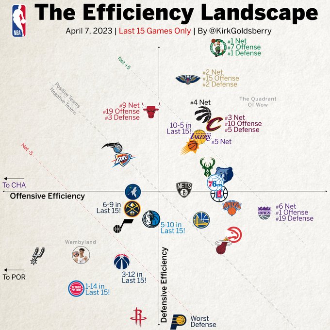
One form of visualization which has become popular is called The Efficiency Landscape, developed by Kirk Goldsberry, an NBA analyst at ESPN.

It takes the form of a scatter plot with $4$ quadrants, depicting defensive efficiency vs. offensive efficiency. See the picture below for an example:

The Efficiency Landscape

The idea is that:

  • Teams in the $1^\text{st}$ quadrant have above average offense and above average defense.
  • Teams in the $2^\text{nd}$ quadrant have below average offense and above average defense.
  • Teams in the $3^\text{rd}$ quadrant have below average offense and below average defense.
  • Teams in the $4^\text{th}$ quadrant have above average offense and below average defense.

Thus, you would expect that teams in the $1^\text{st}$ quadrant are the best, teams in the $2^\text{nd}$ and $4^\text{rd}$ quadrants are worse, and teams in the $3^\text{th}$ quadrant are the worst.

We will adapt this visualization to see if it serves as a good way to classify teams' performance in the playoffs.

We will make a bubble plot of defensive rating (DRtg) vs. offensive rating (ORtg), where the size of the bubble indicates the number of playoff wins.

Considering the NBA's scoring explosion, we will make a separate plot for each season so that the league's rise in scoring efficiency over time does not skew our results (as a confounding variable).

In [ ]:
cols = 4
rows = np.ceil((len(seasons) - 1) / cols).astype(int)

fig = px.scatter(
    past_data,
    x="ORtg",
    y="DRtg",
    size="PlayoffW",
    color="Team",
    facet_col="Season",
    title=f"{data_labels['DRtg']} vs. {data_labels['ORtg']} by {data_labels['Season']}",
    labels=data_labels,
    facet_col_wrap=cols,
    height=1200,
    facet_col_spacing=0.05,
)

fig.update_xaxes(matches=None, showticklabels=True)
fig.update_yaxes(matches=None, showticklabels=True)
fig.for_each_annotation(lambda a: a.update(text=a.text.split("=")[-1]))

None

Now, we will add lines to each plot indicating the median offensive rating (ORtg) and median defensive rating (DRtg) for each season. These lines create our quadrants.

In [ ]:
for index, season in enumerate(seasons[:-1]):

    row = rows - (index // cols)
    col = index % cols + 1

    season_data = past_data[past_data["Season"] == season]

    median_ORtg = season_data["ORtg"].median()
    median_DRtg = season_data["DRtg"].median()

    fig.add_vline(x=median_ORtg, line_width=2, line_color="black", row=row, col=col)
    fig.add_hline(y=median_DRtg, line_width=2, line_color="black", row=row, col=col)

Finally, we can look at the plots.

In [ ]:
fig.show()

We can see that:

  • Teams in the $1^\text{st}$ quadrant tend to have the largest bubbles.
  • Teams in the $2^\text{nd}$ and $4^\text{th}$ quadrants tend to have the next largest bubbles.
  • Teams in the $3^\text{rd}$ quadrant tend to have the smallest bubbles.

This lends credence to the idea that having good offensive efficiency and good defensive efficiency can serve as a good predictor of playoff success.

Note, though, that this trend is not perfect. For example, in $2022$, the Golden State Warriors won the NBA Championship despite being in the bottom-left corner of the $3^\text{rd}$ quadrant, which indicates bad offensive and defensive efficiency.

Perhaps, though, this relation can serve as one of many important factors in our models later on.

4.4. Combining Common Predictors: Seed and True Shooting Percentage

Now, let's combine two of the statistics most commonly used to predict playoff success: seed (Seed) and true shooting percentage (TS%).

We already saw that individually, each of these statistics does show some correlation with playoff wins, but the correlation is not very strong.

Can we get a better prediction by combining these statistics?

That is what we will do below, by creating a density heatmap with seed on the $x$-axis and true shooting percentage (TS%) on the $y$-axis. The color of each tile in the heatmap is determined by computing the average playoff wins (PlayoffW) for a team with the corresponding seed and true shooting percentage.

In [ ]:
fig = px.density_heatmap(
    past_data,
    x="Seed",
    y="TS%",
    z="PlayoffW",
    histfunc="avg",
    title=f"Average {data_labels['PlayoffW']} by {data_labels['Seed']} and {data_labels['TS%']}",
    labels={
        **data_labels,
        f"avg of {data_labels['PlayoffW']}": f"Average {data_labels['PlayoffW']}",
    },
    nbinsx=8,
    text_auto=".0f",
)

hovertemplate = "<br>".join(
    [
        "%{xaxis.title.text}=%{x}",
        "%{yaxis.title.text}=%{y}",
        f"Average {data_labels['PlayoffW']}=%{{z:.2f}}",
    ]
)

fig.update_layout(coloraxis={"colorbar": {"title": "Average Playoff Wins"}})
fig.update_traces(hovertemplate=hovertemplate)

fig.show()

As we can see from the heatmap, looking at seed and true shooting percentage together is quite insightful.

We can see that teams towards the left of the heatmap (i.e. those with higher seeds) and teams towards the top of the heatmap (i.e. those with higher true shooting percentages) tend to have more playoff wins.

For example, almost all of the teams which average more than $8$ playoff wins (i.e. make the conference finals) are either $1^\text{st}$ or $2^\text{nd}$ seeds. The only exceptions are $3^\text{rd}$ and $4^\text{th}$ seeds with true shooting percentage over $58\%$.

This shows that seed and true shooting percentage balance each other out to some degree. Higher-seeded teams can succeed in the playoffs despite poor shooting efficiency, and highly efficient teams can succeed in the playoffs despite low seeding.

Pairing other statistics together in this fashion would likely yield similar results, so it will be important to consider factors together when we build our models.

5. Modeling: Analysis, Hypothesis Testing, & Machine Learning

Now that we have explored some of the trends in the data, we will begin the stages of analysis, hypothesis testing, and machine learning. We will be making extensive use of scikit-learn for machine learning.

5.1. Problem Definition

Let's start off by defining the problem we are trying to solve. As we stated in the introduction, our goal is to predict the outcome of the NBA playoffs using data from the regular season.

First, let's take look at the variables we are using to make our predictions.

In [ ]:
X_names = past_data.columns.tolist()[:-3]

We have the following categorical variables:

In [ ]:
X_categorical_names = X_names[:3]
X_categorical_names
Out[ ]:
['Season', 'Team', 'Conference']

We have the following numerical variables:

In [ ]:
X_numerical_names = X_names[3:]
X_numerical_names
Out[ ]:
['Seed',
 'FG',
 'FGA',
 'FG%',
 '3P',
 '3PA',
 '3P%',
 '2P',
 '2PA',
 '2P%',
 'FT',
 'FTA',
 'FT%',
 'ORB',
 'DRB',
 'TRB',
 'AST',
 'STL',
 'BLK',
 'TOV',
 'PF',
 'PTS',
 'SRS',
 'ORtg',
 'DRtg',
 'NRtg',
 'Pace',
 'FTr',
 '3PAr',
 'TS%',
 'eFG%',
 'TOV%',
 'ORB%',
 'FT/FGA',
 'OppeFG%',
 'OppTOV%',
 'DRB%',
 'OppFT/FGA',
 'Rank',
 'W%',
 'HomeW%',
 'RoadW%',
 'EastW%',
 'WestW%',
 'ConferenceW%']

Now, let's take a look at the variable we are trying to predict:

In [ ]:
y_name = past_data.columns.tolist()[-2]
print(y_name)
PlayoffW

Since playoff wins (PlayoffW) is a continuous variable, this can be classified as a regression problem.

5.2. Splitting Data

Before we can start solving this regression problem, we need to split the data into random train and test subsets.

We can do this using a scikit-learn utility (train_test_split). We will specify a test_size of $0.2$, so $80\%$ of the data will be included in the train split and $20\%$ of the data will be included in the test split. We will also specify a random_state of $0$ to allow for reproducible results.

In [ ]:
X = past_data[X_names]
y = past_data[y_name]
X_train, X_test, y_train, y_test = train_test_split(X, y, test_size=0.2, random_state=0)

5.3. Machine Learning Pipelines

Now, we will build machine learning pipelines to solve this regression problem.

5.3.1. Preprocessing Data

The first step in our machine learning pipelines will be to preprocess the data.

Since there are no missing values in our data, there is no need for imputation.

For our categorical variables (Season, Team, and Conference), we need to encode the values. Specifically, we will use the OneHotEncoder (docs), which turns a categorical variable with $n$ values into an $n$-bit vector.

In [ ]:
categorical_transformer = Pipeline(
    steps=[("encoder", OneHotEncoder(handle_unknown="ignore"))]
)

For our numerical variables, we need to scale the values. There are a few different scalers that might work, so we can try all of them and see which works best:

  • StandardScaler (docs), which standardizes each variable into $Z$-scores
  • MinMaxScaler (docs), which scales each variable to a given range
  • MaxAbsScaler (docs), which scales each variable by its maximum absolute value
  • RobustScaler (docs), which scales each variable using statistics that are robust to outliers
In [ ]:
numerical_transformer = Pipeline(steps=[("scaler", None)])

scalers = [StandardScaler(), MinMaxScaler(), MaxAbsScaler(), RobustScaler()]

Now, we can define our preprocessor step using the ColumnTransformer (docs), which applies the categorical_transformer to our categorical variables and the numerical_transformer to our numerical variables.

In [ ]:
preprocessor = ColumnTransformer(
    transformers=[
        ("categorical", categorical_transformer, X_categorical_names),
        ("numerical", numerical_transformer, X_numerical_names),
    ]
)

preprocessor_params = {"preprocessor__numerical__scaler": scalers}

5.3.2. Feature Selection / Dimensionality Reduction

The second step in our machine learning pipelines will be feature selection / dimensionality reduction. We will use RFECV (docs), which selects features using recursive feature elimination with cross-validation.

We will make our feature_selector a function of the model being used. Thus, when performing RFECV, we will use the specified model as the estimator. It recursively removes the feature ranked least important by the estimator until we have the desired number of features.

This can help us prevent overfitting, so that our model generalizes well to new data and doesn't only perform well on the training data.

Different cross validation splitting strategies could work, so we will try $3$, $5$-, and $10$- fold cross-validation and see what works best.

In [ ]:
def feature_selector(model):
    return RFECV(model)


feature_selector_params = {
    "feature_selector__cv": [3, 5, 10],
}

5.3.3. Model Selection / Hyperparameter Tuning

The third step in our machine learning pipelines is model selection / hyperparameter tuning.

There are a lot of different models we could use to solve this regression problem, so we will try some of them and see what works best. We will also specify different hyperparameters to try out in the learning process.

These are the models we will try:

  • Linear Regression (LinearRegression): ordinary least squares linear regression (minimizes the residual sum of squares)
  • Ridge Regression (Ridge): least squares linear regression with $L_2$ regularization
  • Lasso Regression (Lasso): linear regression with $L_1$ regularization
  • Elastic Net Regression (ElasticNet): linear regression with combined $L_1$ and $L_2$ regularization
  • Decision Tree Regression (DecisionTreeRegressor): models the data as a tree of decision rules
  • Random Forest Regression (RandomForestRegressor): fits decision trees on random subsamples of the data and averages the results
  • Gradient Boosting Regression (GradientBoostingRegressor): additive model where a decision tree is fit on the negative gradient of the loss function in each stage
  • AdaBoost Regression (AdaBoostRegressor): repeatedly fits a decision tree on the same data, with weights being adjusted based on the error of the previous predicion
In [ ]:
models = {
    "Linear Regression": {
        "model": LinearRegression(),
        "params": {},
    },
    "Ridge Regression": {
        "model": Ridge(),
        "params": {"model__alpha": np.logspace(-4, 4, 9)},
    },
    "Lasso Regression": {
        "model": Lasso(),
        "params": {"model__alpha": np.logspace(-4, 4, 9)},
    },
    "Elastic Net Regression": {
        "model": ElasticNet(),
        "params": {
            "model__alpha": np.logspace(-4, 4, 9),
            "model__l1_ratio": np.linspace(0, 1, 11),
        },
    },
    "Decision Tree Regression": {
        "model": DecisionTreeRegressor(),
        "params": {
            "model__criterion": [
                "squared_error",
                "friedman_mse",
                "absolute_error",
                "poisson",
            ],
            "model__max_depth": [3, 5, 10, 15, 20, 25],
            "model__min_samples_split": [2, 5, 10, 15],
        },
    },
    "Random Forest Regression": {
        "model": RandomForestRegressor(),
        "params": {
            "model__n_jobs": [-1],
            "model__n_estimators": [10, 50, 100, 300, 500],
            "model__max_depth": [3, 5, 10, 15, 20, 25],
            "model__min_samples_split": [2, 5, 10, 15],
        },
    },
    "Gradient Boosting Regression": {
        "model": GradientBoostingRegressor(),
        "params": {
            "model__learning_rate": np.logspace(-2, 0, 3),
            "model__n_estimators": [10, 50, 100, 300, 500],
            "model__max_depth": [3, 5, 10, 15, 20, 25],
            "model__min_samples_split": [2, 5, 10, 15],
        },
    },
    "AdaBoost Regression": {
        "model": AdaBoostRegressor(),
        "params": {
            "model__n_estimators": [10, 50, 100, 300, 500],
            "model__learning_rate": np.logspace(-2, 0, 3),
            "model__loss": ["linear", "square", "exponential"],
        },
    },
}

Now, we have everything we need to build our pipelines.

For each of the models we have selected, we will do the following:

  • Build a Pipeline with preprocessor, feature_selector, and model steps. These steps are chained together to form a single model.

    We will use the memory parameter to enable caching and set the verbose parameter to True so we can view progress while the Pipeline is running.

  • Create a param_grid by combining the parameters for the preprocessor, feature_selector, and model steps.

  • Check if we have already fitted the model and saved it for future use using skops.

    • If the model has already been saved, just load it from the .skops file in the models directory. There is no need to retrain the model.

    • If the model has not already been saved, we will do the following:

      • Set up an exhaustive grid search (GridSearchCV).

        We pass in our pipeline and param_grid. The grid_search will exhaustively generate candidates from the param_grid by fitting the pipeline using every permutation of the hyperparameters specified.

        We also pass in a cross-validation scheme (cv). In this case, we are using $5$-fold cross-validation. This involves randomly splitting the training data into $5$ folds, using $4$ for training and $1$ for validation. We repeat this $5$ times and then take the average of the performance metrics. This can help us prevent overfitting, so that our model generalizes well to new data and doesn't only perform well on the training data.

      • Fit the grid search on the training data (X_train and y_train).

        The grid search gives us the model using the set of hyperparameters which has the best performance metrics.

      • Save the fitted model as a .skops file in the models directory.

In [ ]:
# go through each model
for (name, m) in models.items():

    # print model name
    print(f"====== {name} ======")

    # build pipeline
    m["pipeline"] = Pipeline(
        steps=[
            ("preprocessor", preprocessor),
            ("feature_selector", feature_selector(m["model"])),
            ("model", m["model"]),
        ],
        memory="cache",
        verbose=True,
    )

    # build param grid
    m["param_grid"] = {**preprocessor_params, **feature_selector_params, **m["params"]}

    # get path for loading/saving model
    modified_name = name.replace(" ", "")
    path = f"models/{modified_name}.skops"

    # if fitted model has already been saved, load it
    if Path(path).exists():
        with open(path, "rb") as file:
            m["grid_search"] = sio.load(file, trusted=True)
            print(f'Loaded fitted model from "{path}".')

    # otherwise, proceed with fitting model
    else:

        # perform exhaustive grid search with cross-validation
        m["grid_search"] = GridSearchCV(m["pipeline"], m["param_grid"], cv=5, n_jobs=-1)
        m["grid_search"].fit(X_train, y_train)

        # save fitted model
        Path(path).parent.mkdir(parents=True, exist_ok=True)
        with open(path, "wb") as file:
            sio.dump(m["grid_search"], file)
            print(f'Saved fitted model to "{path}".')

    # print new line
    print("\n")
====== Linear Regression ======
Loaded fitted model from "models/LinearRegression.skops".


====== Ridge Regression ======
Loaded fitted model from "models/RidgeRegression.skops".


====== Lasso Regression ======
Loaded fitted model from "models/LassoRegression.skops".


====== Elastic Net Regression ======
Loaded fitted model from "models/ElasticNetRegression.skops".


====== Decision Tree Regression ======
Loaded fitted model from "models/DecisionTreeRegression.skops".


====== Random Forest Regression ======
Loaded fitted model from "models/RandomForestRegression.skops".


====== Gradient Boosting Regression ======
Loaded fitted model from "models/GradientBoostingRegression.skops".


====== AdaBoost Regression ======
Loaded fitted model from "models/AdaBoostRegression.skops".


5.4. Evaluating Models

Now that we have all of our fitted models, let's evaluate them.

5.4.1. Comparing Models

Let's start off by comparing models using performance metrics using performance metrics. We will use the following metrics:

  • Coefficient of Determination ($R^2$): the proportion of the variance of the target variable that is explained by the independent variables in the model (indicates "goodness of fit," with the best possible score being $1.0$)
  • Root Mean Squared Error ($\text{RMSE}$): the square root of the expected value of the squared error loss ($L_2$ norm)
  • Mean Absolute Error ($\text{MAE}$): the expected value of the absolute error loss ($L_1$ norm)

We'll calculate these performance metrics by predicting the target variable using the test data and comparing the real values of the target variable to the predicted values.

In this case, our target variable is playoff wins (PlayoffW).

We will tabulate the results in a DataFrame.

In [ ]:
model_data = pd.DataFrame(
    {
        "Model": [],
        "R2": [],
        "RMSE": [],
        "MAE": [],
    }
)

model_labels = {
    "Model": "Model",
    "R2": "Coefficient of Determination (R2)",
    "RMSE": "Root Mean Squared Error (RMSE)",
    "MAE": "Mean Absolute Error (MAE)",
}

for (name, m) in models.items():

    y_pred = m["grid_search"].predict(X_test)

    row = pd.DataFrame(
        [
            {
                "Model": name,
                "R2": r2_score(y_test, y_pred),
                "RMSE": mean_squared_error(y_test, y_pred, squared=False),
                "MAE": mean_absolute_error(y_test, y_pred),
            }
        ]
    )

    model_data = pd.concat([model_data, row]).reset_index(drop=True)

model_data
Out[ ]:
Model R2 RMSE MAE
0 Linear Regression 0.268811 3.997359 3.266602
1 Ridge Regression 0.445865 3.479894 2.684129
2 Lasso Regression 0.415087 3.575229 2.783280
3 Elastic Net Regression 0.408355 3.595744 2.808841
4 Decision Tree Regression 0.526508 3.216729 2.381250
5 Random Forest Regression 0.436751 3.508393 2.628015
6 Gradient Boosting Regression 0.478939 3.374446 2.606227
7 AdaBoost Regression 0.484823 3.355339 2.521633

Now, let's make a bar plot of model performance. We will have the model on the $x$-axis and the score on the $y$-axis. There will be $3$ bars for each model: $1$ for each performance metric ($R^2$, $\text{RMSE}$, and $\text{MAE}$).

In [ ]:
fig = px.bar(
    model_data,
    x="Model",
    y=["R2", "RMSE", "MAE"],
    title="Model Performance",
    labels=model_labels,
    barmode="group",
    height=600,
)

fig.update_layout(yaxis_title="Score", legend_title_text="Metric")

fig.for_each_trace(
    lambda t: t.update(
        name=model_labels[t.name],
        legendgroup=model_labels[t.name],
        hovertemplate="<br>".join(
            [
                "Model=%{x}",
                "Score=%{y}",
            ]
        ),
    )
)

fig.show()

While many of these models perform well, we can see that one clearly stands out as the best: the decision tree regression model (though gradient boosting regression and AdaBoost regression are close). It happens to have the best performance in all $3$ metrics:

  • $R^2 = 0.5265$ (highest)

    This is a measure of precision. Approximately $52.65\%$ of the variance in playoff wins is explained by the independent variables in the decision tree regression model.

  • $\text{RMSE} = 3.22$ (lowest)

    This is a measure of accuracy that heavily penalizes large errors, making it more sensitive to outliers. By this measure, on average, the decision tree regression model is off by $3.22$ wins when predicting playoff wins.

  • $\text{MAE} = 2.38$ (lowest)

    This is a measure of accuracy that doesn't penalize large errors as much, making it more robust to outliers. By this measure, on average, the decision tree regression model is off by $2.38$ wins when predicting playoff wins.

Based on these scores, the decision tree regression model has moderately high precision (as indicated by the $R^2$ value) and moderately high accuracy (as indicated by the $\text{RMSE}$ and $\text{MAE}$ values).

While there is certainly room for improvement (especially in the $R^2$ value), these are some pretty good results for something notoriously hard to predict.

5.4.2. Diving Deeper

Now that we know the decision tree regression model performs the best, let's take a look at how it works.

Let's start off by taking a look at what features the model uses.

In [ ]:
pipeline = models["Decision Tree Regression"]["grid_search"].best_estimator_
feature_names = pipeline["preprocessor"].get_feature_names_out()
selected_features_mask = pipeline["feature_selector"].get_support()
selected_features = feature_names[selected_features_mask]
selected_features
Out[ ]:
array(['numerical__Seed'], dtype=object)

It turns out that the best decision tree regression model only uses Seed as a feature. All of the other features were removed during the feature selection / dimensionality reduction process.

Was this the case for all of the models we trained?

In [ ]:
for (name, m) in models.items():
    m_pipeline = m["grid_search"].best_estimator_
    m_feature_names = m_pipeline["preprocessor"].get_feature_names_out()
    m_selected_features_mask = m_pipeline["feature_selector"].get_support()
    m_selected_features = m_feature_names[m_selected_features_mask]
    print(f"====== {name} ======")
    print(m_selected_features)
    print("\n")
====== Linear Regression ======
['categorical__Season_2003' 'categorical__Season_2004'
 'categorical__Season_2005' 'categorical__Season_2006'
 'categorical__Season_2007' 'categorical__Season_2008'
 'categorical__Season_2009' 'categorical__Season_2010'
 'categorical__Season_2011' 'categorical__Season_2012'
 'categorical__Season_2013' 'categorical__Season_2014'
 'categorical__Season_2015' 'categorical__Season_2016'
 'categorical__Season_2017' 'categorical__Season_2018'
 'categorical__Season_2019' 'categorical__Season_2020'
 'categorical__Season_2021' 'categorical__Season_2022'
 'categorical__Team_Cleveland Cavaliers'
 'categorical__Team_Detroit Pistons'
 'categorical__Team_Golden State Warriors'
 'categorical__Team_Los Angeles Lakers' 'categorical__Team_Miami Heat'
 'categorical__Team_New Jersey Nets' 'categorical__Team_Sacramento Kings'
 'numerical__FG' 'numerical__FGA' 'numerical__FG%' 'numerical__3P'
 'numerical__3PA' 'numerical__2P' 'numerical__2PA' 'numerical__FT'
 'numerical__FTA' 'numerical__ORB' 'numerical__DRB' 'numerical__TRB'
 'numerical__PTS' 'numerical__ORtg' 'numerical__DRtg' 'numerical__NRtg'
 'numerical__eFG%' 'numerical__W%' 'numerical__HomeW%' 'numerical__RoadW%']


====== Ridge Regression ======
['categorical__Team_Cleveland Cavaliers'
 'categorical__Team_Golden State Warriors'
 'categorical__Team_Los Angeles Lakers' 'categorical__Team_Miami Heat'
 'numerical__Seed' 'numerical__FT%' 'numerical__NRtg' 'numerical__TOV%']


====== Lasso Regression ======
['numerical__Seed' 'numerical__NRtg' 'numerical__OppFT/FGA'
 'numerical__Rank']


====== Elastic Net Regression ======
['numerical__Seed' 'numerical__SRS' 'numerical__NRtg'
 'numerical__OppFT/FGA' 'numerical__Rank']


====== Decision Tree Regression ======
['numerical__Seed']


====== Random Forest Regression ======
['numerical__Seed' 'numerical__DRtg' 'numerical__Rank']


====== Gradient Boosting Regression ======
['categorical__Season_2021' 'categorical__Team_Cleveland Cavaliers'
 'categorical__Team_Golden State Warriors'
 'categorical__Team_Los Angeles Lakers' 'categorical__Team_Miami Heat'
 'categorical__Team_San Antonio Spurs' 'numerical__Seed' 'numerical__FG'
 'numerical__FGA' 'numerical__FG%' 'numerical__3PA' 'numerical__3P%'
 'numerical__2P' 'numerical__2PA' 'numerical__FT' 'numerical__FTA'
 'numerical__FT%' 'numerical__ORB' 'numerical__TRB' 'numerical__AST'
 'numerical__BLK' 'numerical__TOV' 'numerical__PF' 'numerical__PTS'
 'numerical__SRS' 'numerical__ORtg' 'numerical__DRtg' 'numerical__NRtg'
 'numerical__3PAr' 'numerical__TS%' 'numerical__eFG%' 'numerical__TOV%'
 'numerical__ORB%' 'numerical__FT/FGA' 'numerical__OppeFG%'
 'numerical__OppTOV%' 'numerical__OppFT/FGA' 'numerical__Rank'
 'numerical__W%' 'numerical__HomeW%' 'numerical__RoadW%'
 'numerical__EastW%' 'numerical__WestW%' 'numerical__ConferenceW%']


====== AdaBoost Regression ======
['numerical__Seed' 'numerical__DRtg' 'numerical__eFG%' 'numerical__Rank'
 'numerical__HomeW%' 'numerical__ConferenceW%']


As we can see, it's actually the case that only the decision tree regression model uses a single feature. The rest of the models use more features, but they have worse performance on the test data.

This is not necessarily a bad thing. Perhaps, Seed truly is the best predictor of playoff wins, and the other features do not contribute significantly to the predictive power of the model.

The simplicity of the decision tree regression model is quite nice, and we can actually visualize how it works.

In [ ]:
plot_tree(
    pipeline["model"],
    feature_names=selected_features,
    class_names=[y_name],
    filled=True,
    rounded=True,
)
Out[ ]:
[Text(0.4583333333333333, 0.875, 'numerical__Seed <= -0.429\nsquared_error = 22.424\nsamples = 256\nvalue = 5.328'),
 Text(0.25, 0.625, 'numerical__Seed <= -0.869\nsquared_error = 19.849\nsamples = 97\nvalue = 9.402'),
 Text(0.16666666666666666, 0.375, 'numerical__Seed <= -1.308\nsquared_error = 16.996\nsamples = 66\nvalue = 10.606'),
 Text(0.08333333333333333, 0.125, 'squared_error = 19.877\nsamples = 31\nvalue = 10.161'),
 Text(0.25, 0.125, 'squared_error = 14.114\nsamples = 35\nvalue = 11.0'),
 Text(0.3333333333333333, 0.375, 'squared_error = 16.264\nsamples = 31\nvalue = 6.839'),
 Text(0.6666666666666666, 0.625, 'numerical__Seed <= 0.45\nsquared_error = 7.692\nsamples = 159\nvalue = 2.843'),
 Text(0.5, 0.375, 'numerical__Seed <= 0.01\nsquared_error = 10.188\nsamples = 65\nvalue = 4.492'),
 Text(0.4166666666666667, 0.125, 'squared_error = 10.462\nsamples = 30\nvalue = 5.067'),
 Text(0.5833333333333334, 0.125, 'squared_error = 9.429\nsamples = 35\nvalue = 4.0'),
 Text(0.8333333333333334, 0.375, 'numerical__Seed <= 0.889\nsquared_error = 2.784\nsamples = 94\nvalue = 1.702'),
 Text(0.75, 0.125, 'squared_error = 4.379\nsamples = 30\nvalue = 2.567'),
 Text(0.9166666666666666, 0.125, 'squared_error = 1.521\nsamples = 64\nvalue = 1.297')]

We can observe a simple tree-like structure, in which a team is assigned a certain number of playoff wins based on its seed.

This simple model manages to outperform the other models, which rely on many more features than just Seed.

5.4.3. Predicting the $2023$ NBA Playoffs

Now, it's time to put this decision tree regression model to the test by using it to predict the outcome of the $2023$ NBA Playoffs.

Let's start off by generating the predictions and sorting teams by predicted playoff wins (PredPlayoffW).

In [ ]:
decision_tree = models["Decision Tree Regression"]["grid_search"]

X_current = current_data[X_names]
current_pred = X_current.copy()
current_pred["PredPlayoffW"] = decision_tree.predict(X_current)
current_pred = current_pred[["Team", "Conference", "Seed", "PredPlayoffW"]]
current_pred = current_pred.sort_values(by="PredPlayoffW", ascending=False)
current_pred = current_pred.reset_index(drop=True)

current_pred
Out[ ]:
Team Conference Seed PredPlayoffW
0 Boston Celtics East 2 11.000000
1 Memphis Grizzlies West 2 11.000000
2 Milwaukee Bucks East 1 10.161290
3 Denver Nuggets West 1 10.161290
4 Sacramento Kings West 3 6.838710
5 Philadelphia 76ers East 3 6.838710
6 Phoenix Suns West 4 5.066667
7 Cleveland Cavaliers East 4 5.066667
8 Golden State Warriors West 5 4.000000
9 New York Knicks East 5 4.000000
10 Los Angeles Clippers West 6 2.566667
11 Brooklyn Nets East 6 2.566667
12 Atlanta Hawks East 8 1.296875
13 Los Angeles Lakers West 7 1.296875
14 Minnesota Timberwolves West 8 1.296875
15 Miami Heat East 7 1.296875

Now, let's rank these teams within their conferences by the predicted number of playoff wins and assign a status (PlayoffStatus) indicating how far they are expected to go in the playoffs based on their rank relative to other teams.

In [ ]:
current_pred["ConferencePlayoffRank"] = (
    current_pred.groupby("Conference")["PredPlayoffW"]
    .rank(ascending=False, method="first")
    .astype("int64")
)


def playoff_status(row):
    if row["ConferencePlayoffRank"] <= 1:
        return "Finals"
    elif row["ConferencePlayoffRank"] <= 2:
        return "Conference Finals"
    elif row["ConferencePlayoffRank"] <= 4:
        return "Conference Semifinals"
    elif row["ConferencePlayoffRank"] <= 8:
        return "First Round"


current_pred["PlayoffStatus"] = current_pred.apply(playoff_status, axis=1)

current_pred
Out[ ]:
Team Conference Seed PredPlayoffW ConferencePlayoffRank PlayoffStatus
0 Boston Celtics East 2 11.000000 1 Finals
1 Memphis Grizzlies West 2 11.000000 1 Finals
2 Milwaukee Bucks East 1 10.161290 2 Conference Finals
3 Denver Nuggets West 1 10.161290 2 Conference Finals
4 Sacramento Kings West 3 6.838710 3 Conference Semifinals
5 Philadelphia 76ers East 3 6.838710 3 Conference Semifinals
6 Phoenix Suns West 4 5.066667 4 Conference Semifinals
7 Cleveland Cavaliers East 4 5.066667 4 Conference Semifinals
8 Golden State Warriors West 5 4.000000 5 First Round
9 New York Knicks East 5 4.000000 5 First Round
10 Los Angeles Clippers West 6 2.566667 6 First Round
11 Brooklyn Nets East 6 2.566667 6 First Round
12 Atlanta Hawks East 8 1.296875 7 First Round
13 Los Angeles Lakers West 7 1.296875 7 First Round
14 Minnesota Timberwolves West 8 1.296875 8 First Round
15 Miami Heat East 7 1.296875 8 First Round

Based on this decision tree regression model, we would predict that the Boston Celtics and the Memphis Grizzlies are the teams most likely to make it to the finals, with the model predicting that both teams will win roughly $11.00$ playoff games.

The $2023$ NBA Playoffs are still ongoing, but we can see that this model is not fully accurate. For example, the Memphis Grizzlies were eliminated in the first round, winning just $2$ games, despite the model's prediction that they would make it to the finals.

Nonetheless, it will be interesting to see how our predictions compare to the actual results once the playoffs are over.

6. Interpretation: Insight & Policy Decision

Now that we have gone through all the other stages of the data science pipeline, it is time to interpret our results and provide insights.

Our goal in this project was to see if we could identify factors underlying teams' level of success in the playoffs. With this information, we wanted to see if we could accurately predict the number of playoff games a team would win given regular season data.

To accomplish this, we went through the following steps:

  • Data Collection: We scraped data from various pages on Basketball Reference for each season.
  • Data Processing: We merged all the data, cleaned it, and made it suitable for analysis.
  • Exploratory Data Analysis & Visualization: We explored trends in the data to get an idea of how we might go about predicting playoff wins.
  • Modeling: Analysis, Hypothesis Testing, & Machine Learning: We built machine learning pipelines using several different models, tuned their hyperparameters through exhaustive grid searches, and evaluated model performance against test data.

In the end, our best model ended up being a decision tree regression model using Seed as its only feature. The model accounted for approximately $53\%$ of the variance in playoff wins (as measured by $R^2$) and was accurate to within $2$ or $3$ games (as measured by $\text{MAE}$ and $\text{RMSE}$, respectively).

While it was surprising to see that a model with just $1$ feature ended up having the best performance, it was insightful in the sense that it indicated how crucial seeding is in determining playoff success: the teams that do the best in the regular season tend to do the best in the playoffs. The other features don't provide much additional information, considering how much variance there is in the data.

This result also highlights the difficulty in predicting playoff wins using only regular season data. There is so much variability within a season that statistics don't reflect:

  • Injuries
  • Trades
  • Team chemistry
  • Coaching
  • Etc.

Making predictions about the NBA is extremely difficult, and even the experts get it wrong. That being said, it can still be interesting to see different ways of going about predicting the NBA playoffs.

If you'd like to see another, more rigorous, approach, you can check out FiveThirtyEight's live-updating $2022\text{-}23$ NBA Predictions. They make their forecasts by simulating the season, taking into account individual player performance as well as factors like injuries, trades, and changes in player performance throughout the season. There projections can be surprisingly accurate sometimes, but even they get things wrong from time to time.

To conclude, hopefully you enjoyed learning about how we can predict the outcome of the NBA playoffs with reasonable precision and accuracy by going through the stages of the data science pipeline! We can make predictions about other things by going through the same steps, though the specific techniques might vary depending on the problem we are trying to solve.